|
|
|
|
The many gain picture...
|
In the previous section we
examined a function called the logistic function and observed
that its graph depended on the parameter we called gain. As the
gain increased, the height of the graph (its amplitude)
increased. You may think of adjusting the gain parameter as
though you were turning the volume control on your stereo. In
fact parameters like gain are sometimes called control
parameters. Review this function and the effect of gain by
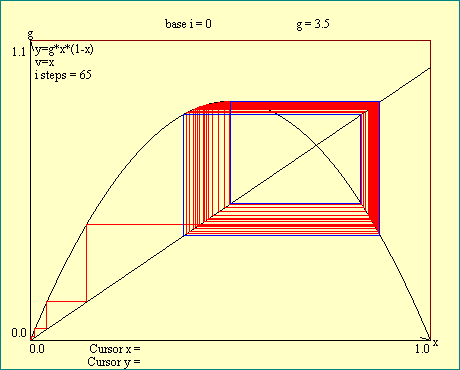
playing around with the
Attractor Demonstration
display.
In the function graphs displayed in the last section, we
picked a value of gain and then varied the independent variable
x, calculating and plotting the dependent variable y at each x
location. What we propose now is to pick a value for the
independent variable x and hold it fixed. Then vary the control
parameter gain and plot the dependent variable at each g
location. This in effect interchanges the role of parameter and
independent variable. This exchange of variables will allow us to
see the effect on the function of iterating from at a particular
point with a whole set of gain values.
If we carry out the scheme described above for the logistic
function, what would the graph look like? The logistic function
is
y=g*x*(1-x)
We have restricted our exploration to a domain of x to be greater than 0 and less than
1. Let us take any x in that interval, say 0.5, and hold it as a constant in the function so
y=g*0.5(1-0.5)
Multiplying this out we get
y=g*0.25
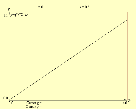
This is a pretty simple result. It says if x is 0.5, y is 1/4 of the gain. If we picked some
other x, y would still be a fixed fraction of the gain. The graph would be a straight line.
|
|
|
The effect of varying the initial value of x, x0, may be seen
in the next display. You will see the slope of the straight line
map is controlled by x0. You will also notice that increasing x0
from 0.5 or decreasing it from 0.5 has the same effect. This
follows from the symmetry about the line
x=0.5
of the logistic function. For low iteration numbers the map clearly depends on the value of
x0. Run the
Phase-Control Maps
display, varying x0 between 0 and 1 with the iteration control set to iteration zero to
illustrate what we were saying. We will begin referring to iterations by number at this
point. The zeroth iteration, symbolized by i0, is just the function itself. i1 is the first
iteration, i2 the second and so on.
This plot of y vs. gain is given the name phase-control map.
This hyphenated name comes from the two dimensions of the map.
The horizontal axis now represents the control parameter rather
than the independent variable. The vertical axis still represents
the dependent variable but the term phase is applied to that
dimension of the map. This terminology arises from the study of
dynamical systems that we will get into later. In effect we have
created a new space measured in dimensions of gain and the
unitless number y, a phase-control space. We take the domain of
the phase-control map to be 0<g<4 since this covers the
kind of behavior we want to demonstrate.
|
|
The logistic function itself,
y0=g*x0*(1-x0)
is zeroth iteration, i0. For the first iteration, i1,
y1=g*x1*(1-x1)
remembering that iterating means x1=y0. Substituting y0 for x1 gives us:
y1=g * (g*x0*(1-x0)) * (1-(g*x0*1-x0))
So y1 depends only on g and x0. By multiplying this out and rearranging you can see:
y1=g^2*(x0-x0^2)-g^3*(x0-x0^2)^2
To get our map we fixed the value of x0 at some number between 0 and 1, so x0-x0^2 is just
some positive constant less than 1, call it "u". Now y1 may be written:
y1=u*g^2-u^2*g^3
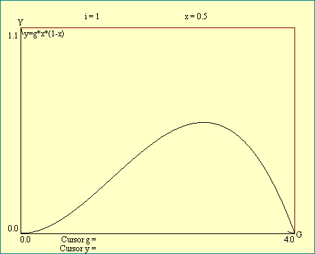
In i0, y depended only on the first power of g. in i1, y depends on the second and third
power of g. The map of i0 was just a straight line. The map of i1 bends upward for small
values of g then downward as the negative term takes over. Remember for g<1 small powers
of g are larger than high powers of g.
|
|
|
Run the
Phase-Control Maps
display again and explore the effect of initial x value on iterates higher than zero.
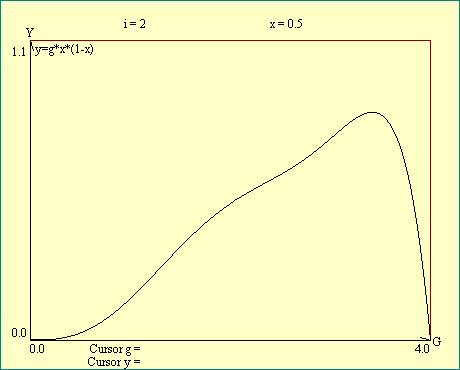
For i2 the dependence on g is given by the following
mess:
y2=u*g^3-u^2*g^4-u^2*g^5+2*u^3*g^6-u^4*g^7
 I suspect that in general the pattern we detect in the i2 expression holds for
higher iterates, but it is too hard for me to verify that the first term of the
nth iteration (in) will involve g^(n+1). The last term will involve g^(2^n+n+1).
There will be
2^n+1 terms with coefficients decreasing as power of g increases
and a mixture of plus and minus signs. In any event it is evident that the
complication of the expression goes up exponentially.
|
|
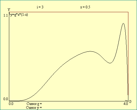
The implication of this explosion of complexity for maps of higher iterations is
troubling. Remember that our assumption in graphing was that the function was
well behaved in the region we were trying to plot. You will see that at the
higher values of g the map becomes more and more jagged as the iteration number
increases. Imagine what the map of the 500th iteration or the 5000th might look
like. These functions of g would be so badly behaved that a graph even
with a very high resolution, that is with the domain divided into very many
steps, could not accurately reflect the function. There would be points on the
function completely missed by the graph. Run the Phase Control Maps
display one more time.
|
|
|
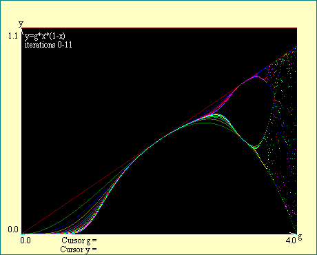
Now we want to extend our phase-control map to look at several
iterations at one time. This is done by picking a value of gain
corresponding to each pixel all the way across the display and
carrying out the iteration as often as desired using that gain.
For each iteration between the first and last to be plotted the y
value is plotted above the chosen gain. Then we move to the next
gain value and repeat the whole process. Each calculated point is
marked by a lighted pixel of color based on the iteration.
For the higher iteration
numbers, depending on your computer, you might begin to notice
that the plot takes longer to develop. In fact since Java is an
interpreted language, requiring a lot of the work to be done at
run time, we are going to push the system pretty hard with some
of the later displays. If you are curious about this stuff and
want to see a full powered (fast) version, try our
Order program.
Run the Quadratic Iterations i0-i11
display next. These first 12 iterations begin to display some of
the interesting characteristics of the logistic phase-control
map. Think about the features of this map and try to reason out
why you see what you do. We will be examining the details of this
map as we get into the next section. Some folks are surprised by
the complexity inherent in iterating the simple logistic
function. You should not be surprised at this point because you
have seen that iteration produces complex equations.
In the next lesson we will explore the phase control map of
the logistic function in more detail.

Are there any questions?
|

 Next Next
 Previous Previous
 Other Other
|
|
|
|


