|
Up and away... both... together... at the same time...
|
In trying to pin down the location of a particle in a
reference frame, we were led into the swamp of vector arithmetic so to speak. Let's try
at this point to pick up the thread of our story. We are still
dealing with the kinematics of a single particle here but we have
relaxed the 1 dimensional restriction applied earlier. For the
time being let's restrict ourselves to a two dimensional
space since the ideas are the same and the third dimension
complicates the pictures. As we did in the 1 dimensional case, we
will first work with the general relationships among particle
position, velocity and acceleration, then consider the special
case of constant acceleration in order to get at some simple
equations describing the particle motion.
In our discussion of functions we
identified an independent and a dependent variable, then related
one to another through a function. This led to a graphical
representation of the function. For example we plotted
x=10*t-t2. In physics, we are going to want to predict
the future so our interest will be in expressing each of the
parameters of particle motion as a function of time, making time
the independent variable and things like position , velocity and acceleration the dependent
variables.
When we introduced the idea of a
rate of change
of a dependent variable with respect to an independent
variable, the initial example was speed being the rate of change
of distance with respect to time. So we have already seen one
instance of time being the independent variable. Distance and
speed are scalar quantities. The vector equivalents are
"displacement" and "velocity", including the
direction intelligence along with the magnitude. Displacement is defined as a
change in position which we remember is the difference between
two vectors, an initial position and a final position. I
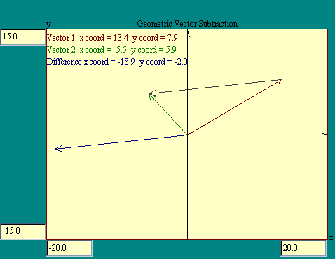
illustrated this in the vector subtraction display. If the
vectors r1 and r2
represent an initial and final position then the vector Dr = r2 -
r1 represents a displacement. The use of
r to represent position in more than 1 dimension is common
in the literature, possibly derived from radius being the
distance from a center to a point. Take another look at the
Geometric Vector Subtraction
display.
|
|
|
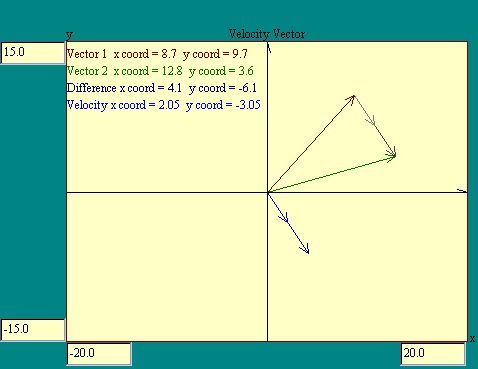
How then would we calculate the velocity from the displacement
vector? By analogy to the speed formula, we can write a
definition of velocity as velocity = displacement / time.
Remembering the italics for vectors convention,
v =
Dr / Dt.
We know how to divide a vector by a scalar. We just divide each
of the vector's scalar components by the scalar t, where the
value of t we use is really a Dt, the
time difference between when the particle was at
r1 and when it was at r2.
In the next display,
Velocity Vector ,
you may calculate velocities based on a fixed Dt of 2.0 seconds. Use the cursor and mouse
button to mark the position vectors r1 and
r2.
You should have noticed that the velocity vector was in the
same direction as the displacement vector and was half the
length. The direction of course was the same as the displacement
because division by a scalar does not alter a vector's
direction even thought it may reverse the sense of the vector.
The length of the velocity vector depends not only on the size of
Dt but also on the scale of our
reference frame coordinate system.
We have been assuming that the units on our position and
displacement vectors were meters so that the values along the
axes represented meters of distance. In calculating velocity, we
divided by time, yielding units of meters per second. Nothing
requires that the same scale on the screen apply to meters per
second as to meters but as a matter of convenience unless
specified otherwise we will use the same scale factor.
|
|
Now consider a particle moving along
some arbitrary path in our reference frame. Since the path is
arbitrary we may not assume that the velocity is constant or even
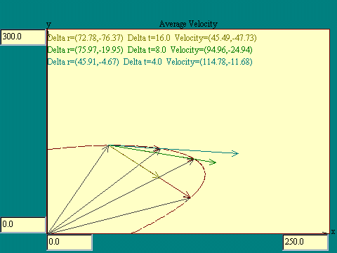
changing in any regular way. In the Average
Velocity display you will see that the velocity vector
calculated over any finite interval of time is really the average
velocity over that time. At any instant between the initial and
final time, the velocity vector might be different in either
direction or magnitude or both. Notice that the length of the
displacement vector, Dr, is
always shorter than the actual path over which the particle
travels. This should tell you something about the relationship of
the magnitude of the average velocity and the average speed of
the particle.
|
|
|
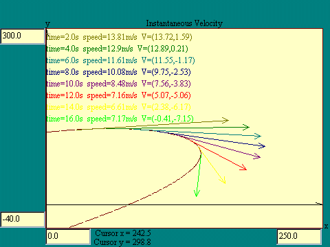
As you could see by going to
smaller and smaller Dt on the Average
Velocity display, the velocity approaches a limit as Dt approaches zero. This is the
instantaneous velocity of the particle at the point on its path
marked by the velocity vector. The direction of the instantaneous
velocity is tangent to the
curve at that instant. Run the Instantaneous
Velocity display to see this illustrated. Notice that the
word "speed" is used to denote the magnitude of the
velocity.
|
|
I indicated that the path of the particle was marked with time
ticks because the time dependence of the particle's position
was not visible in the chosen reference frame. This is a
complication which deserves a bit of exploration.
Suppose that a particle is following some particular path
through space. We should make a careful distinction between the
graph of y as a function of the independent variable x, and a
curve traced out by a moving particle in two dimensional space.
The two plots might look the same but in the first case the value
of x determines the value of y. In the second case the position
of the particle is a function of time. The fact that the position
has an x and a y component actually ties the x and y values
together so that they are not independent of each other but the
relationship is not one of independence and dependence.
What does it mean to say that a position vector, call it
r, is a function of time? Well just like y being a function
of x meant that there was some rule relating to every x some
value of y, r being a function of time means that there
is some rule relating to every value of time, t, a value for
r. But the vector r may be expressed in terms of
its component vectors like this,
r = x *  + y * + y *  ,
where ,
where  and and  are the unit vectors which
are constant, meaning they are independent of time. So when we
say the position vector r is a function of time we are
actually saying that x and y are each functions of time. are the unit vectors which
are constant, meaning they are independent of time. So when we
say the position vector r is a function of time we are
actually saying that x and y are each functions of time.
In physics we may know, or be able to figure out, what the
rule is relating each of the variables x and y to time. We could
then plot x as a function of time on one graph and y as a
function of time on another using time as the independent
variable in each case. Then the relationship between x and y
would be fixed, without us ever having to express it directly.
This trick of using another variable, time in this case, to get
at the relationship between x and y so as to plot the path of a
particle is called a "parametric " representation of
the particle path and the functions relating x to time and y to
time are called parametric equations.
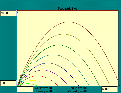
To illustrate the application of
parametric equations, let's look at the case of a particle
whose horizontal position changes with time like
x = vx * t
and whose vertical position changes with time like
y = vy * t - 4.9 * t2.
To see the path of such a particle run the
Parametric Plot
display. In our parametric plotting example we began with the
horizontal and vertical positions as known functions of time.
Quite often we will not know these functions explicitly. Later in
this course we will be determining the time dependent behavior of
various system parameters.

Are there any questions?
|
|
|
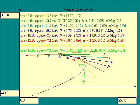
Now let's return to looking at
our particle on its arbitrary path and explore the acceleration
it is experiencing. Remember that acceleration is the rate of
change of velocity with respect to time.
a =
Dv / Dt
Run the Average Acceleration display to
see the relationship among displacement, velocity and
acceleration.
The instantaneous acceleration is developed from the average
through the limiting process in which we look at smaller and
smaller time intervals between adjacent velocity vectors. The Instantaneous Acceleration display shows
the instantaneous velocity and corresponding instantaneous
acceleration vectors at a series of times along the particle
path.
The unit of length is the meter, so displacement is in meters.
Velocity is calculated as displacement divided by time so its
units are meters per second. Acceleration is calculated as
velocity divided by time so its units are meters per second per
second, or meters per second squared. Now we will return to the
idea of constant acceleration applied to 2 dimensions.
|
|
 This may be a good place to talk a bit
about choosing appropriate reference frames. Careful attention to
which way is x can save a lot of work. When we say we will have a
constant acceleration in 2 dimensions, that means that the
acceleration is constant in both magnitude and direction. We
could choose the directions of the axes without regard to the
direction of the acceleration vector. If we did, in general the
acceleration would have a component along each dimension. Having
to keep track of the motion in such an out of whack reference
frame adds a lot of complication to the arithmetic. This may be a good place to talk a bit
about choosing appropriate reference frames. Careful attention to
which way is x can save a lot of work. When we say we will have a
constant acceleration in 2 dimensions, that means that the
acceleration is constant in both magnitude and direction. We
could choose the directions of the axes without regard to the
direction of the acceleration vector. If we did, in general the
acceleration would have a component along each dimension. Having
to keep track of the motion in such an out of whack reference
frame adds a lot of complication to the arithmetic.
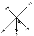
Suppose for example that the -y axis
of the reference frame made an angle q
with the direction of the constant acceleration like this. Then
the equation describing motion in the x direction would be
x = x0 + v0x * t + 1/2
* ax * t2,
where we have just copied the
1 dimensional constant acceleration
results from before. The symbol v0x is the component of initial velocity in the
x direction. The symbol ax is the component of the
acceleration vector a in the x direction. That component
is given by the expression
ax = -|a| * sin(q).
Putting that all together we get
x = x0 + v0x * t + 1/2
* -|a| * sin(q) *
t2.
Going through a similar process for motion in the y dimension we
get
y = y0 + v0y * t + 1/2
* -|a| * cos(q) *
t2.
|
|
|
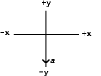
The preceeding mess is something we
could well do without. Let's see what happens to the these
equations when we straighten up the reference frame so that the
-y axis lies along the acceleration vector as shown here. The
effect of this is to make the angle q
equal to zero. Then sin(q) = 0 and
cos(q) = 1. Putting those values into
the former expressions for motion in the x and y dimensions we
get
x = x0 + v0x * t and y
= y0 + v0y * t -1/2 * |a| *
t2.
As you can see, proper choice of reference frame makes life
easier. We will return to this idea later.
|
|
In our discussion of reference frames I
slipped in a significant idea without making much fuss about it.
In looking at constant acceleration in 2 dimensions, I used a
result from our 1 dimensional discussion - twice - once in the x
dimension and once in the y dimension. It may not be obvious to
you that it is legitimate to treat the x and y motion of a single
particle as two instances of 1 dimensional motion. Think of it
this way. Any acceleration in the x direction can only change the
x direction velocity since the change in velocity is just the
acceleration times Dt and Dt is a scalar. Likewise velocity in the x
direction can only change x direction position for the same
reason. So as long as the accelerations along each dimension are
independent, so are the velocities and positions. We may consider
systems where the accelerations in different dimensions are
coupled in some way, but that is a complication we will save for
later.
So for constant acceleration in 2 dimensions (or 3 dimensions
for that matter) when the reference frame is chosen sensibily and
there are no weird connections between accelerations in different
dimensions, we can adopt the results of our 1 dimensional
constant acceleration study directly. In particular let's
look at a particle under the influence of the Earth's
gravity. We have already established that gravity near the
surface of the Earth provides a practically constant acceleration
straight down of 9.8 m/s2 so one of our reference
frame axes should lie in that direction. I will place the -y axis
in the direction of the gravitational acceleration, consistent
with common practice.
Fixing the y axis with gravity, vertically, locks in our 2
dimensional (plane) reference frame to a plane perpendicular to
the Earth's surface. The other vector we need to accomodate
in the plane is the initial velocity. So we orient the reference
frame so as to contain the initial velocity vector. The x axis
then is a horizontal line in the plane defined by the
acceleration vector and the initial velocity vector. Now that we
have built our reference frame, just place it so that the
particle lies in the plane and we are ready to examine the
particle's motion. As long as our assumption of constant
(unchanging in either magnitude or direction) acceleration is
true, the particle, wherever it may go, will not wander out of
the reference frame plane.
At this point your physics text
probably has lots of examples of what is called "projectile
motion". They all come down to the application of the laws
we worked out for 1 dimensional, constant acceleration, motion
applied separately to the x and y dimensions of the reference
frame. The key to these problems is to take the given information
which usually boils down to an initial velocity vector and
resolve the initial velocity into its x and y components. Those
components then are the initial velocities to be used in the
equations describing the x and y motion.
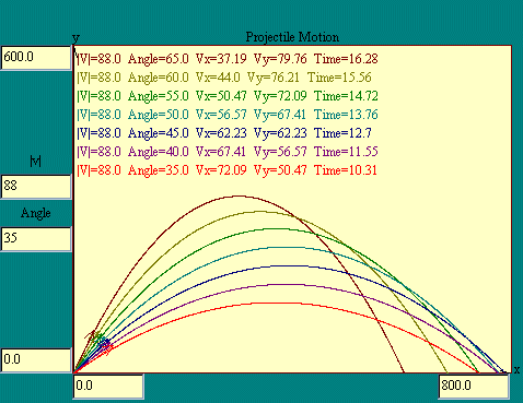
The
Projectile Motion
display automatically solves projectile motion problems for you once you
sift the initial velocity vector out of the given information.
You should recognize it as similar to the Parametric Plot display
shown earlier. Play around with this display to build up your
intuition about projectile motion.
|
|
|
In some physics texts you may find at this point some more
kinematics, involving uniform circular motion and multiple
reference frames. We will hold off on discussion of these topics.
Uniform circular motion will be covered after we get to know
something about the relationship between force and motion.
Multiple reference frames will be covered in the section on the
nature of space.
At this point there is a choice to be made about how to get at
the laws of nature. One approach is to come in at a very profound
level which involves the interaction of space and matter, and
some sort of "least action" principle, following the
trail blazed by Lagrange and Hamilton. The advantage of this way
is that the laws of nature fall out logically from a single
assumption. The disadvantage is that this requires a degree
mathematical sophistication that would take us a long time to
establish from the base we have built so far. If you are curious
you may try our
Physics_T
runtime book to fill in some of the background behind Newton's laws of motion.
The other approach is to develop the laws of nature from the
common sense which grows out of experience. It was Sir Isaac
Newton who first expressed this common sense in formal terms. The
advantage of this approach is that our intuition about nature is
consistent with this development. The disadvantage is that more
of the facts of dynamics are considered to be laws, requiring us
to remember more and understand less. Also the connections among
the various laws are not necessarily obvious. We will take the
Newtonian tack at this point.
Are there any questions?
|

 Next
Previous
Other
Next
Previous
Other
|